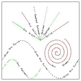
Previous Chapter LLUs Home Next Chapter IndexThere are several methods for drawing lines and curves (polylines) on a plot and controlling line characteristics, like the dash pattern, color, width, and smoothness. The following modules demonstrate how to draw curves and set their characteristics using GKS, SPPS, and higher level routines.
------------------------------------------------------------------
Parameter  Brief description     Fortran type    Routines affected
------------------------------------------------------------------
PB         Polyline Buffer size  Integer (2-50)  PLOTIF
------------------------------------------------------------------
-------------------------------------------------------------------------
Parameter  Brief description              Fortran type  Routines affected
-------------------------------------------------------------------------
IPAU       Line and gap size              Integer       DASHDC, DASHDB
FPART      First solid segment factor     Real          DASHDC
IGP        Character GaP flag             Integer       DASHDC
ICLOSE     Pen-up parameter               Integer       DASHDC, DASHDB
IOFFS      Smoothing flag                 Integer       DASHDC
TENSN      TENSioN factor                 Real          DASHDC
NP         Point-interpolation parameter  Integer       DASHDC
SMALL      Saved points min. distance     Real          DASHDC
L1         Max. number of points saved    Integer       DASHDC
ADDLR      Number of free space units     Real          DASHDC
ADDTB      Number of free space units     Real          DASHDC
MLLINE     Max. crowded-LINE length       Integer       DASHDC
-------------------------------------------------------------------------
CALL SETUSV (PNAM, IVAL)
This module demonstrates how to set the line type and how to draw lines using GKS routines.

1       REAL    XCD(1500), YCD(1500)
2       CALL GSPLCI (2)
3       DO 40 ING=1,1500
4          RAD=REAL(ING)/1000.
5          ANG=DTR*REAL(ING-1)
6          XCD(ING)=.25+.5*RAD*COS(ANG)
7          YCD(ING)=.25+.5*RAD*SIN(ANG)
8  40   CONTINUE
9       CALL SET (.24,.37,.48,.61,-1.,1.,-1.,1.,1)
10      CALL GPL(1500, XCD, YCD)
11      CALL SET (.03,.10,.43,.50,-1.,1.,-1.,1.,1)
12      CALL GPL(1500, XCD, YCD)
CALL GPL (NPTS, XCD, YCD)
Line 1 defines the X and Y input coordinate arrays.
Line 2 sets the current polyline color index to 2. The color table and associated indices were set up prior to entering this code segment.
Lines 3 through 8 compute the X and Y input coordinates for a spiral line.
Line 9 calls the SET routine to define the mapping from the fractional coordinate system of the plotter to the user coordinate system. This effectively positions the spiral on the frame off the coast of Southeast Asia.
Line 10 calls GPL to draw the spiral. The first argument specifies that there are 1,500 coordinates in the line. The second and third arguments are the arrays of coordinates defining the spiral.
Line 11 defines a new mapping and effectively positions the second spiral off the east coast of Africa.
Line 12 draws the second spiral.
This module demonstrates how to draw lines using the LINE routine.
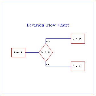
1       CALL GSPLCI(2)
2       CALL SET (0.,1.,0.,1.,0.,20., 0.,20.,1)
3       CALL GSLWSC(4.)
4       CALL LINE(2.,8.,2.,10.)
5       CALL LINE(2.,10.,5.,10.)
6       CALL LINE(5.,10.,5.,8.)
7       CALL LINE(5.,8.,2.,8.)
8       CALL PLCHLQ(3.5,9.,'Read I',15.,0.,0.)
CALL LINE (X1, Y1, X2, Y2)
The fspline.f code segment draws a single box and places the text "Read I" in its center.
Line 1 sets the current polyline color index. A color table was set up previously in the code using the GKS GSCR routine. Line 2 sets up a mapping between the plotter coordinates and the user coordinate system. Line 3 sets the line width to 4. Lines 4 through 7 make four calls to the LINE routine to draw the four sides of a box. Line 8 draws the text, "Read I", in the center of the box that was just drawn.
This module demonstrates how to draw curves using CURVE and compares it with the GKS routine GPL.
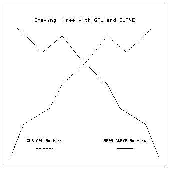
1  DATA XCOORD/1.,2.,3.,5.,7.,9.,13.,16.,19.,23./
2  DATA YCOORD/1.,3.,5.,6.,7.,10.,13.,16.,14.,17./
3
4  CALL SET (0.,1., 0., 1., 25., 0., 0., 20., 1)
5  CALL GSLN(2)
6  CALL GPL(10,XCOORD,YCOORD)
7  CALL GSLN(1)
8  CALL CURVE(XCOORD,YCOORD,10)
9  CALL FRAME
CALL CURVE (XCD, YCD, NPTS)
The code segment and graphic demonstrate how to use the CURVE routine and how it differs from the GKS curve-drawing routine, GPL.
If the routine SET is called to reverse the axes or use logarithmic mappings, then you should use the CURVE routine instead of GPL, since GPL does not recognize axis reversal or logarithmic mappings.
In the fspcurve example, CURVE and GPL plot the same data points. However, since the SET call reversed the X axis, GPL does not draw the curve correctly.
Lines 1 and 2 of the fspcurve.f code segment initialize the X and Y coordinates of the line to be drawn.
Line 4 sets up the mapping from plotter space to user coordinates. Notice that we have reversed the X axis to map from 25 to 0.
Line 5 sets the line type to "dashed" using the GKS GSLN routine. GSLN takes a single integer argument, which specifies the type of line to be drawn. The argument may be one of the following:
Line 6 calls the GKS routine GPL to draw a dashed line. GPL will ignore the axis reversal specified with the SET call.
Line 7 sets the line type to "solid."
Line 8 calls the SPPS routine CURVE to draw a solid line. CURVE recognizes the axis reversal and therefore mirrors the curve drawn by the GPL routine.
Line 9 advances the frame.
This module demonstrates how to draw curves using CURVED and set line characteristics such as color and width.
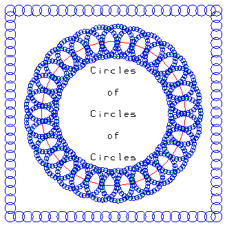
1       REAL XCOOR2(120), YCOOR2(120)
2
3       CALL SET(.01,.99,0.01,.99,0.,1.,0.,1.,1)
4       CALL GNCRCL(.5,.5,.333,30,XCOOR2, YCOOR2)
5       CALL GSLWSC(5.)
6       CALL GSPLCI(2)
7       CALL CURVED(XCOOR2,YCOOR2,30)
8       CALL PLCHLQ(.5,.7,'Circles',.03,0.,0.)
9       CALL PLCHLQ(.5,.6,'of',.03,0.,0.)
10      CALL PLCHLQ(.5,.5,'Circles',.03,0.,0.)
11      CALL PLCHLQ(.5,.4,'of',.03,0.,0.)
12      CALL PLCHLQ(.5,.3,'Circles',.03,0.,0.)
CALL CURVED (XCD, YCD, NPTS)
The fdlcurvd.f code segment and graphic demonstrate how to use the CURVED routine and set line characteristics like color and line width. Every circle in the graphic was drawn with a call to CURVED. The code segment draws the large circle in which the text "Circles of Circles of Circles" is centered. Although CURVED was used only to draw circles in this example, it can be used to draw curves of any shape.
Line 1 declares the array of user coordinates. Line 3 sets up the mapping between the plotter and user coordinates. In this example, the user coordinates range from 0. to 1. in both the X and Y directions. Line 4 calls a routine that initializes the XCOOR2 and YCOOR2 arrays with the coordinates of a circle centered at (.5,.5), a radius of .333, and 30 points, which define it. Line 5 sets the line width to 5 (1 is the default). Line 6 sets the color of the line. The color table was set up prior to entering this code segment with the GKS GSCR routine. The argument (2) passed to the GSPLCI routine represents an index in the color table. Line 7 draws the large circle in the center of the graphic. Lines 8 through 12 draw text in the center of the large circle.

1       STR = '$''$''Line''drawn''with''VECTD$''$''$''$'''
2       CALL DASHDC(STR,15,20)
3       CALL FRSTD(0.,.60)
4       DO 22 I=1,360
5              Y = (SIN(REAL(I)*(TWOPI/360.)) * .25) + .60
6              CALL VECTD(REAL(I)/360.,Y)
7   22  CONTINUE
8       STR = '$$$$$$Line''drawn''with''CURVED$$$$$$$$$$$$'
9       CALL DASHDC(STR,15,20)
10      DO 23 I=1,360
11              XCOORD(I) = REAL(I)/360.
12              YCOORD(I) = (SIN(REAL(I)*(TWOPI/360.)) * .25) + .45
13  23  CONTINUE
14      CALL CURVED(XCOORD, YCOORD, 360)
15      CALL DASHDB(63903)
16      CALL LINED(0.1,.15, .9,.15)
17      CALL PLCHLQ (0.5,0.10,'Line drawn with LINED' ,20.,0.,0.)
      CALL DASHDC (CPAT, JCRT, JSIZE)
      CALL DASHDB (IPAT)
The fdldashd.f code segment and graphic demonstrate how to set the dash pattern and line label of a line using DASHDC and DASHDB.
Line 1 initializes a string that specifies a dash pattern. Dollar signs ($) represent solid portions and single quotation marks (') represent spaces. Note that since FORTRAN77 string constants are enclosed in single quotation marks ('), a single quotation mark (') is represented by two adjacent single quotation marks, (''). Line 2 sets the dash pattern and specifies that the length of a line or space represented by the dollar sign ($) or single quotation mark (') is 15 plotter address units. The last argument specifies the character width in the line label to be 20 plotter address units.
Line 3 calls the FRSTD routine to put the plotter pen down at a point specified in world coordinates. FRSTD must be called prior to calling VECTD to position the plotter pen. This represents the starting point of a line segment drawn by the VECTD routine.
Lines 4 through 7 draw a dashed sine curve using the VECTD routine. VECTD takes two arguments, the X and Y world coordinates of the new plotter pen position. Line 8 initializes a string with a new dash pattern. Line 9 sets the dash pattern. Lines 10 through 13 specify the coordinates for the second sine curve. Line 14 draws the second curve using CURVED.
Line 15 sets a new dash pattern using DASHDB. 63903 (decimal) = 1111100110011111 (binary); therefore, line 15 specifies a dashed line with unequal lengths of solid portions and gaps. Line 16 draws a straight line with the LINED routine. LINED takes four arguments. The first two are the X and Y world coordinates of the starting point of the line, and the second two are the X and Y world coordinates of the ending point of the line. Line 17 draws a label under the last line.
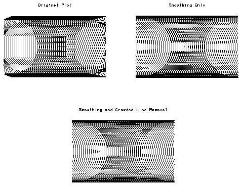
1       REAL XCOORD(10), YCOORD(10)
2
3       CALL RESET
4       DO 10 I=1,50
5              CALL GNCRCL(REAL(I)/50.,.5,.333,10,XCOORD, YCOORD)
6              CALL CURVED(XCOORD,YCOORD,10)
7   10  CONTINUE
8       CALL PLCHLQ(.5,.95,'Smoothing and Crowded Line Removal',.02,0.,0.)
9       CALL FRAME
CALL RESET
The three graphics on the opposite page demonstrate the effect of smoothing and crowded-line removal. The effects of curve smoothing are obvious in this example. However, the effects of crowded-line removal are harder to detect. The lines are most crowded along the top and bottom of the plot. If you look closely at the third image, you will notice some of the crowded lines that are present in the two previous images have been removed, especially near the top and bottom of the plot.
Smoothing is turned on by loading the libdashsmth.o library when you link your program. This is done by adding the -smooth option to your ncargf77 command line:
ncargf77 -smooth file.for by explicitly loading libdashsmth.o when you compile:
f77 file.f $NCARG_ROOT/lib/ncarg/robj/libdashsmth.o ...Crowded-line removal and smoothing are turned on by loading the libdashsupr.o library when you link your program. This is done by adding the -super option to your ncargf77 command line:
ncargf77 -super file.for by explicitly loading libdashsupr.o when you compile your program:
f77 file.f $NCARG_ROOT/lib/ncarg/robj/libdashsupr.o ...Each of the three example graphics was generated from the same source code, but the last two graphics were compiled with the -smooth and -super options, respectively. The first graphic was created without using any options.
Line 1 of the fdlsmth.f code segment declares the X and Y coordinate arrays that will contain the user coordinates for drawing the curves. Line 3 calls RESET to initialize the plot buffer. This call was only needed for the last graphic, which used crowded-line removal. If we only wanted to do curve smoothing, the RESET routine could have been omitted. Lines 4 through 7 draw 50 circles across the frame. In this example, we call CURVED. However, line smoothing and crowded-line removal work with the VECTD routine also. Smoothing does not effect the output of the LINED routine, but crowded-line removal does. Line 8 labels the plot. Line 9 advances the frame.
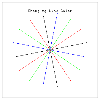
1       CALL GSCR (1,0,1.,1.,1.)
2       CALL GSCR (1,1,0.,0.,0.)
3       CALL GSCR (1,2,1.,0.,0.)
4       CALL GSCR (1,3,0.,1.,0.)
5       CALL GSCR (1,4,0.,0.,1.)
6       DTHETA = TWOPI/NPTP
7       DO 10 I=1,16
8          ANG = DTHETA*REAL(I) + .19625
9          XC = RP*COS(ANG)
10         YC = RP*SIN(ANG)
11         CALL GSPLCI (MOD(I,4)+1)
12         CALL GSLWSC(6.)
13         CALL LINED(X0P,Y0P,X0P+XC,Y0P+YC)
14  10  CONTINUE
      CALL GSCR (WKID, CI, CR, CG, CB)
      CALL GSPLCI (INDEX)
Lines 1 through 5 in the fgklnclr.f code segment call the GSCR routine to create a color table with five entries (indices 0 through 4). Line 1 defines the background color white (CR=1., CG=1., CB=1.) Lines 2, 3, 4, and 5 define the colors black, red, green, and blue, respectively. Line 6 initializes a constant. Line 7 enters a loop that draws 16 lines. Line 8 computes the line angle. Lines 9 and 10 compute the endpoint of a line. Line 11 sets the line color by specifying an index into the color table created by GSCR. Line 12 sets the line width. Line 13 draws the line. Line 14 ends the loop.
More information on color tables appears in Chapter 7 "Color tables and color mapping systems."
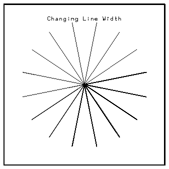
1       DO 10 I=1,16
2          ANG = DTHETA*REAL(I) + .19625
3          XC = RP*COS(ANG)
4          YC = RP*SIN(ANG)
5          CALL GSPLCI (1)
6          CALL GSLWSC(REAL(I))
7          CALL LINED(X0P,Y0P,X0P+XC,Y0P+YC)
8   10  CONTINUE
CALL GSLWSC (WIDTH)
The fgklnwth.f code segment shows how the lines were drawn by increasing the line width on every iteration of the loop.
Line 1 begins the loop. Line 2 computes the line angle. DTHETA is a constant used to space the lines equally around a circle, and it is defined before entering the loop. Lines 3 and 4 compute the endpoint of a line. Line 5 sets the line color. Line 6 sets the line width. Line 7 draws a single line, and line 8 completes the loop.
Previous Chapter LLUs Home Next Chapter Index